Week of 11/20/2017 - Progress Report 6

Tamara Jovanovic
Nov 22, 2017
5 min read

Topics covered: Setting Up Optical System, Obtaining Laser Power Readings, Obtaining Laser Spectra

Materials used: Collimators, post holders, posts, collimator mounting bracket, collimator holder, single-mode fiber, clamping forks, cuvette, cuvette stand, YOKOGAWA OSA, Newport Universal Fiber Optic Detector, FemtoSecond Laser, Optical Laser Safety Goggles

For this week’s objective, we wanted to set up the optical system and see if we can get any data using the optical components, including getting power readings and spectra.

First, the system was set up as pictured below. The collimators were set to face each other on the posts, and through the collimator mounting brackets. The first collimator’s input was connected to the laser output. Both posts were lowered as much possible, to ensure that the height of the system doesn’t vary. By using the IR card and with the lights off, we could see a little red dot through the collimator, which meant that the laser was working.

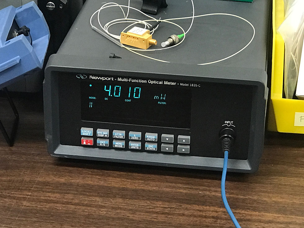
We wanted to check how much power the laser light was emitting, so we put the fiber coming out of the laser into the Newport Universal Fiber Optic Detector, as shown below. What we got was a power reading of 4.010 mW (milliWatts). This is the full power of the laser output. Theoretically, when the laser was shined through the first collimator and the light was captured by the second one, the fiber coming out of the second collimator should still give us a power reading, but attenuated from the original power reading.

Since we were still unfamiliar with the distance that needed to be set between the collimators, we started experimenting with catching the laser light with the second collimator at various distances between the two posts. The IR card was used to make sure that the light was perfectly aligned in the middle of the second collimator.

Since getting power readings through 2 collimators was almost impossible, we lowered the unit scale. The readings were now acquired in nW (nanoWatts). The laser input was still attached to the first collimator, and the fiber coming out of the second collimator was put into the fiber optic power detector. The maximum reading acquired was 208.82 nW.

Pictured below is the OSA when the output of the laser was connected directly to the OSA input. The shape of this spectrum was used as a reference as to how the spectrum should look at the output of the setup described above.

Once we verified through power detection, that we could get an optical output from the coupled collimator setup, we connected the output of the second collimator directly to the spectrometer. This was the most rigorous part of this entire process. For the majority of this week’s attempts, all that was read by the OSA was noise. The first step to progress was shown when the lenses of the 2 spectrometer were pressed against one another manually. This showed hints of the shape of the picture above, albeit very very noisy. Nonetheless, this was enough to show that by very careful and precise adjustment, the output of the setup could generate a clear spectrum.

Therefore, the first attempt to fine adjustment is pictured below.

As seen above, the distance between the collimators is unreasonable, since in the future, cuvettes and their corresponding stand would not fit in between to be able to capture glucose spectra. However, after rigorous turning of the dials on both of the collimators, eventually the OSA showed hints of the laser spectrum, as seen below. However, after several more attempts of fine tuning, the quality of the produced spectrum did not improve. Therefore, instead we proceeded to increase the distance between the 2 collimators to make the setup more practical.

Once again, there was an abundance of rigorous dial turning and repositioning of the collimator mounts in order to generate at least parts of the laser spectrum. Once some progress was noted, the best spectrum for this collimation distance is pictured below.

As seen above, and on the generated spectrum for the short distance collimation attempt, the best we were able to produce was about 30% of the shape of the original laser’s spectrum, but significantly noisy. Therefore, as a final attempt to note significant progress, for the final setup, a temporary cuvette stand was placed in between the collimators to see if the clear walls of the cuvette worsened the quality of the spectrum. The setup is shown below.

Very surprisingly, the setup above greatly improved the spectrum shown on the OSA. After repositioning the cuvette stand a few times, we were able to seemingly reproduce the spectrum of the laser.

After turning on the markers on the OSA, the peak of the produced spectrum showed as -59.09 dBm at 1578.1 nm. Similarly, the peak of the original laser’s spectrum was -20.22 dBm at 1579.2 nm. Therefore, directly from the laser to the OSA, the optical gain is of approximately 0.1. From the result of the setup with the cuvette between the collimators, the optical gain shows approximately 0.001. Therefore, from the results gathered on the OSA, there is approximately a 90% loss of power when the system filters the laser through our setup. Going back to the power detection readings, the maximum power we were able to detect was 208.8 nW from an original 4-4.2 mW. That shows close to complete loss of power through our system.

In order to verify that all of the work described above was not due to lucky observations, multiple trials were performed for the progress noted. However, after multiple attempts for power detection and OSA readings, we could not get the values and spectra to be better than the ones shown above. Therefore, this was the best that could be recorded this week.

PROBLEMS: After this week, there were several problems to note for the current setup, techniques, and procedures taken. First, adjusting the collimators and fine tuning the dials takes a long time. In order to even generate the noisy parts of the spectra shown, it took several hours of rigorous adjustments to achieve. Additionally, even when the spectra are clear or more acceptable, the setup is still very sensitive. For example, when we thought that we had achieved a good positioning, slightly bumping the optical table reverted all progress and noise was shown. The same can be said about meddling with the fiber cords.

Second, there seems to be a significant amount of power loss when the laser light is filtered through our system. As discussed above, the best we were able to capture was approximately a 90% loss of power from the laser. Though the spectrum was clear and virtually the same shape as the spectrum from the laser directly, 90% is a lot and should be discussed further.

The third problem has to do with the practicality of our project in the weeks to come. As previously shown, the laser spectrum can be reproduced when a cuvette is used between the collimators. However, after capturing that spectrum, the cuvette was filled with DI water. The result shown on the OSA was pure noise. Therefore, the most obvious conclusion that came to mind was that water has a highly interfering absorption spectrum at 1550 nm, which is a problem since that wavelength is the basis for this project.

Nonetheless, the entire progress made this week was accomplished by the 3 of us solely, without physical help from any experienced person in optics. Therefore, perhaps these problems have easy solutions, or simply require more thought and discussion.

Nonetheless due to our inexperience with optics this was the current progress we have accomplished. Therefore perhaps these problems have simple solutions that we can ask from an experienced person in optics, or simply we need to more thought and discussion.

Plans For Next Week: