Week of 10/30/2017 - Progress Report 4

Topics Covered: GUI cleanup, Cross Correlation Analysis

Materials: Matlab (v. 2014b or newer)

Summary: Last week, user interface was made easy with the GUI, and 2 methods were started to analyze absorption spectra of acetylene absorption. This week, the GUI was made more user friendly with regards to the project by updating a few already-implemented options and also adding a few others. For example, previously, the GUI looked as shown below:

As shown, the starting wavelength (‘Start WL’) and ending wavelength (‘End WL’) options were preset in pop-up menus as for the user to choose as they like. However, more efficiently and far more viable would be for the user to be able to input the start and end wavelengths as they please. Using the following Matlab code, that was possible.

The variable ‘s1’ stores the first part of the OSA command that sets the start/end wavelengths, and the variable ‘handles.swe’ is used when sending the actual command to the OSA. Another change that was made to the GUI was the plotting options after data is retrieved. Previously, as shown below, the user was given the option to show absorption spectra or absorption lines by pressing two buttons.

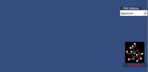
Now, as shown below, the same results can be obtained but using a pop-up menu, which is both simpler and more professional-looking.

Also, as shown on the first picture, the GUI looked ugly because of lots of static text at the bottom. Now, a ‘Help’ menu option was implemented in order to display the same information. This allows the GUI to look cleaner, sleeker, and more professional. The results are shown below.

Before Help Menu is Pressed

After Help Menu is Pressed

Finally, the last technical update that was made to the GUI was adding Reference options. For example, when data is retrieved from the OSA and displayed on the GUI, the plot has nothing to be referenced to in order to compare its validity. Now, after data is retrieved, the user has the option to display a reference plot along with the data. On the same menu option, the user has the option to save recently retrieved data to the reference, in order to use that data as reference. The following code is what makes it possible.

As shown, there will be an excel spreadsheet on the Matlab directory that stores the reference data. When the user navigates to Options>Reference>Get Reference, the following code executes, plotting both the data from the reference and the data retrieved from the OSA on the same axes. If the user navigates to Options>Reference>Save as Reference, the data retrieved from the OSA is stored into the ‘ref.csv’ spreadsheet. Pressing ‘Get Reference’ shows the following result.

Finally, an aesthetic update was made to the GUI. Previously, maximizing the GUI window displayed the plot small compared to the window, and also the buttons/menus and plot went out of place and looked unprofessional. Now, the plot axes was increased in size and the other options were repositioned. The end result looks as follows, showing a more professional-looking GUI when maximized.

In addition to updating the GUI, another new method for analyzing absorption spectra was implemented- Cross Correlation Coefficient between 2 sets of data. Cross Correlation Coefficient performs convolution of 2 signals and generates a coefficient value (0-1) that determines how similar the 2 signals are. This is similar to the RMSE% method previously studied in that the 2 sets of data are compared by a numerical value. However, the beneficial aspect of Cross Correlation Coefficient is that it is calculated by multiplying each point in one of the sets to all the points in the other set individually, and the process is repeated for every single point in the first set. This ensures that every value in the 2 signals are compared directly, getting a more accurate coefficient than RMSE%. Using the ‘xcorr’ built-in Matlab function, a generated set of data from the OSA can be compared to the stored reference data in the GUI. Using acetylene absorption values from the OSA, the following Cross Correlation Coefficient Analysis was performed.

Cross Correlation Coefficient of 0.9992

As shown, generating the same absorption data with different resolution options generates a very high Cross Correlation Coefficient, which is expected since the data is virtually the same. Running the same analysis with completely different data would ideally generate very low coefficients. This method could be useful by having a basis for what acceptable coefficients would be (i.e. know what coefficient values correspond to acceptable matching data). However, the problem that this method poses is the same as RMSE%. The problem is that this coefficient does not distinguish between discrepancies in the x or y axis, so data cannot be completely interpreted from this value. Similarly, there will have to be a method that distinguishes between differences in the x and y axes.

Plans for Next Week:

1. ThorLabs sent our components last week, so the optical setup will be ready.

2. Glucose solutions will be prepared for absorption spectroscopy using our new setup.

3. We now have 3 absorption analysis techniques (Peak Absorption Strength Analysis, RMSE%, and Cross Correlation Coefficient). Additional techniques will need to be researched in order to find solutions for the problems each pose.

4. Attempt to perform current analysis on glucose readings to arrive at conclusions regarding our techniques.

5. Continue updating GUI…